Lesson 4 - Optimal Transport and Schrödinger Bridges

11 Jan 2024 in Lectures Last modified at: 2025-12-31

What Schroedinger has to do with moving dirt

Optional reading for this lesson Permalink

• Peyré & Cuturi - Computational Optimal Transport
• Léonard - A survey of the Schrödinger problem and some of its connections with optimal transport
• De Bortoli et al. - Diffusion Schrödinger Bridge
• Optimal Transport Notes (Cambridge)
• Marco Cuturi - Optimal Transport Primer (3h video)

Slides Permalink

Video (soon) Permalink

In this lecture, we explore the deep connections between optimal transport theory, Schrödinger bridges, and stochastic differential equations. We start with the Schrödinger bridge problem—a question about the most likely path of a diffusion process—and discover how it naturally connects to optimal transport through entropic regularization. This unified framework provides powerful tools for generative modeling, sampling, and domain adaptation in modern machine learning.

• Optional reading for this lesson
• Slides
  • Video (soon)
• 1. The Schrödinger Bridge Problem
  • 1.1 Problem Formulation
  • 1.2 Solution via h-Transform
  • 1.3 Why This Matters for Machine Learning
• 2. From Schrödinger Bridges to Optimal Transport
  • 2.1 The Monge Problem (1781)
  • 2.2 The Kantorovich Relaxation (1940s)
  • 2.3 Entropic Regularization: The Bridge Between Two Worlds
  • 2.4 The Unification: Schrödinger Bridge as Entropic OT
  • 2.5 Dynamic Formulation: Benamou-Brenier
• 3. Solving the Schrödinger Bridge: Iterative Proportional Fitting
  • 3.1 The IPF Algorithm: Detailed Derivation
  • 3.2 Discrete Case: Sinkhorn Algorithm
  • 3.3 Convergence and Properties
• 4. Generative Modeling via Schrödinger Bridges
  • 4.1 Learning Schrödinger Bridges with Neural Networks
  • 4.2 Diffusion Schrödinger Bridges: Score-Based Approach
  • 4.3 DSB Matching: Implementing IPF in Continuous Time
  • 4.4 Practical Considerations for Generative Modeling
• 5. Sampling and Bayesian Inference
  • 5.1 The Sampling Problem in Bayesian Inference
  • 5.2 Stochastic Gradient Langevin Dynamics
  • 5.3 Maximum Likelihood Approach to Schrödinger Bridges
  • 5.4 Practical Sampling from Schrödinger Bridges
  • 5.5 Advantages of Schrödinger Bridges for Sampling
• 6. Domain Adaptation and Transport
  • 6.1 Domain Adaptation via Optimal Transport
  • 6.2 Applications
• 7. Future Directions and Open Questions
  • 7.1 Scalable Algorithms
  • 7.2 Neural Optimal Transport
  • 7.3 Conditional Bridges
  • 7.4 Multi-Marginal Problems
  • 7.5 Geometric Deep Learning
• Credits

1. The Schrödinger Bridge Problem Permalink

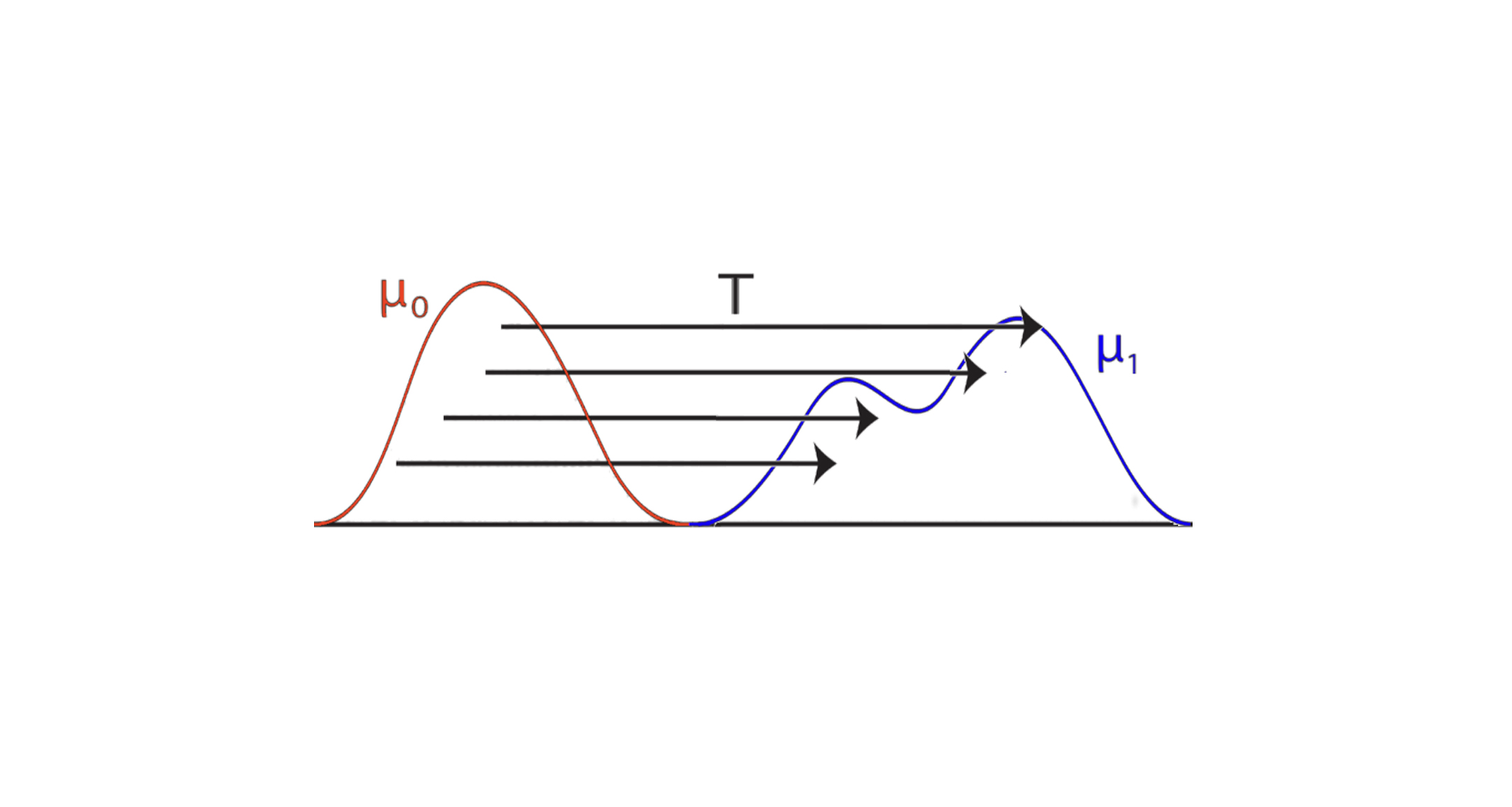
We begin with a problem introduced by Erwin Schrödinger in 1931: given the initial and final marginals $\mu_0$ and $\mu_1$ of a diffusion process, what is the most likely path that the process could have taken? This seemingly abstract question turns out to have profound implications for modern machine learning.

1.1 Problem Formulation Permalink

Consider a reference diffusion process (e.g., Brownian motion) on the time interval $[0,1]$: $$dX_t = b(X_t, t) dt + \sigma dW_t$$

with initial distribution $X_0 \sim \mu_0$. The Schrödinger bridge problem seeks a new process: $$dX_t = \tilde{b}(X_t, t) dt + \sigma dW_t$$

with the same diffusion coefficient $\sigma$ but a modified drift $\tilde{b}$, such that:

• $X_0 \sim \mu_0$ (initial constraint)
• $X_1 \sim \mu_1$ (final constraint)
• The process minimizes the relative entropy (KL divergence) with respect to the reference process

The relative entropy between two path measures $\mathbb{Q}$ and $\mathbb{P}$ is defined as: $$\mathcal{H}(\mathbb{Q} \| \mathbb{P}) = \mathbb{E}_{\mathbb{Q}}\left[\log \frac{d\mathbb{Q}}{d\mathbb{P}}\right]$$

if $\mathbb{Q} \ll \mathbb{P}$ ($\mathbb{Q}$ is absolutely continuous with respect to $\mathbb{P}$), and $+\infty$ otherwise.

1.2 Solution via h-Transform Permalink

The solution to the Schrödinger bridge problem can be expressed using the h-transform we saw in the previous lecture. Specifically, the optimal drift is: $$\tilde{b}(x, t) = b(x, t) + \sigma^2 \nabla_x \log \psi(x, t)$$

where $\psi(x, t)$ is a solution to the Schrödinger system of PDEs: $$\begin{align} \partial_t \psi(x, t) + b(x, t) \cdot \nabla_x \psi(x, t) + \frac{\sigma^2}{2} \Delta_x \psi(x, t) &= 0 \quad \text{(backward Kolmogorov equation)} \\ \partial_t \hat{\psi}(x, t) - \nabla_x \cdot (b(x, t) \hat{\psi}(x, t)) + \frac{\sigma^2}{2} \Delta_x \hat{\psi}(x, t) &= 0 \quad \text{(forward Kolmogorov equation)} \end{align}$$

with boundary conditions:

• $\psi(x, 1) = 1$ for all $x$ (terminal condition for backward equation)
• $\hat{\psi}(x, 0) = \mu_0(x)$ for all $x$ (initial condition for forward equation)
• The product $\psi(x, t) \hat{\psi}(x, t) = p_t(x)$ gives the marginal density at time $t$

Derivation via Variational Calculus: The optimal drift can be derived by considering the first-order optimality conditions for the constrained optimization problem. Using Lagrange multipliers $\lambda_0(x)$ and $\lambda_1(x)$ for the marginal constraints, the Euler-Lagrange equations yield the Schrödinger system.

Connection to h-Transform: The connection becomes clear when we write the transition density of the bridge process: $$p_{t \mid 0}(x_t \mid x_0) = \frac{\psi(x_t, t)}{\psi(x_0, 0)} p^R_{t \mid 0}(x_t \mid x_0)$$

where $p^R_{t \mid 0}$ is the transition density of the reference process. This is exactly the h-transform formula, where $h(x, t) = \psi(x, t)$ serves as the harmonic function that modifies the reference process to satisfy the boundary conditions.

Uniqueness: Under mild regularity conditions (e.g., the reference process has positive transition densities), the Schrödinger system has a unique solution, ensuring the uniqueness of the bridge process.

1.3 Why This Matters for Machine Learning Permalink

The Schrödinger bridge problem provides a principled framework for several key ML tasks:

• Generative Modeling: Bridge from a simple noise distribution to complex data distributions
• Sampling: Transport samples from a tractable prior to an intractable posterior
• Domain Adaptation: Smoothly transport samples between different domains
• Interpolation: Create smooth paths between distributions

By constraining both endpoints, we obtain a unique, optimal transport path that minimizes the “effort” (measured by KL divergence) required to transform one distribution into another. This variational characterization ensures that the bridge process is the most likely path connecting the two distributions under the reference measure.

2. From Schrödinger Bridges to Optimal Transport Permalink

The connection between Schrödinger bridges and optimal transport is profound. As the noise level $\sigma \to 0$, the Schrödinger bridge converges to the optimal transport solution. Understanding this connection reveals why entropic regularization is so powerful.

2.1 The Monge Problem (1781) Permalink

The original optimal transport problem, formulated by Gaspard Monge, asks: given two probability measures $\mu_0$ and $\mu_1$ on $\mathbb{R}^d$, find a transport map $T: \mathbb{R}^d \to \mathbb{R}^d$ that pushes $\mu_0$ forward to $\mu_1$ (i.e., $T_\# \mu_0 = \mu_1$) while minimizing the transport cost: $$\mathcal{M}(\mu_0, \mu_1) = \inf_{T: T_\# \mu_0 = \mu_1} \int c(x, T(x)) d\mu_0(x)$$

where $c(x, y)$ is a cost function. Common choices are:

• Quadratic cost: $c(x, y) = \frac{1}{2}\|x - y\|^2$ (leads to 2-Wasserstein distance)
• Linear cost: $c(x, y) = \|x - y\|$ (leads to 1-Wasserstein distance)

The pushforward notation $T_\# \mu_0$ means that for any measurable set $A$, we have $\mu_1(A) = \mu_0(T^{-1}(A))$, or equivalently, for any test function $f$: $$\int f(y) d\mu_1(y) = \int f(T(x)) d\mu_0(x)$$

2.2 The Kantorovich Relaxation (1940s) Permalink

The Monge problem may not have a solution (the infimum might not be attained, or the constraint $T_\# \mu_0 = \mu_1$ may be too restrictive). Léonard Kantorovich relaxed this by considering transport plans (couplings) instead of transport maps.

A coupling $\gamma$ is a joint probability measure on $\mathbb{R}^d \times \mathbb{R}^d$ with marginals $\mu_0$ and $\mu_1$, meaning:

• $\int_{y \in \mathbb{R}^d} d\gamma(x, y) = d\mu_0(x)$ (first marginal)
• $\int_{x \in \mathbb{R}^d} d\gamma(x, y) = d\mu_1(y)$ (second marginal)

The Kantorovich problem is: $$W_p(\mu_0, \mu_1)^p = \inf_{\gamma \in \Gamma(\mu_0, \mu_1)} \int_{\mathbb{R}^d \times \mathbb{R}^d} \|x - y\|^p d\gamma(x, y)$$

where $\Gamma(\mu_0, \mu_1)$ is the set of all couplings with marginals $\mu_0$ and $\mu_1$. The value $W_p(\mu_0, \mu_1)$ is called the $p$-Wasserstein distance.

For $p=2$, we get the 2-Wasserstein distance $W_2$, which has particularly nice properties:

• It metrizes weak convergence of probability measures
• It has a dynamic formulation (Benamou-Brenier)
• It connects naturally to SDEs and diffusion processes

2.3 Entropic Regularization: The Bridge Between Two Worlds Permalink

The connection between Schrödinger bridges and optimal transport emerges through entropic regularization. Instead of solving the exact Kantorovich problem, we add an entropy penalty: $$W_p^\epsilon(\mu_0, \mu_1)^p = \inf_{\gamma \in \Gamma(\mu_0, \mu_1)} \left\{ \int \|x - y\|^p d\gamma(x, y) + \epsilon \mathcal{H}(\gamma \| \mu_0 \otimes \mu_1) \right\}$$

where $\mathcal{H}(\gamma \| \mu_0 \otimes \mu_1)$ is the relative entropy with respect to the product measure $\mu_0 \otimes \mu_1$, and $\epsilon > 0$ is a regularization parameter.

As $\epsilon \to 0$, the entropically regularized problem converges to the original optimal transport problem: $$\lim_{\epsilon \to 0} W_p^\epsilon(\mu_0, \mu_1) = W_p(\mu_0, \mu_1)$$

2.4 The Unification: Schrödinger Bridge as Entropic OT Permalink

The Schrödinger bridge problem is exactly the entropically regularized optimal transport problem! This is a profound connection that unifies two seemingly different problems.

Theorem (Léonard, Mikami): The Schrödinger bridge problem with reference process $dX_t = \sigma dW_t$ (Brownian motion) and regularization parameter $\epsilon = \sigma^2$ is equivalent to the entropically regularized optimal transport problem with quadratic cost.

Unified Formulation: Let us see how these two threads merge. Consider:

1. Optimal Transport (Kantorovich): Minimize transport cost over couplings: $W_2(\mu_0, \mu_1)^2 = \inf_{\gamma \in \Gamma(\mu_0, \mu_1)} \int \|x - y\|^2 d\gamma(x, y)$

2. Entropic Regularization: Add entropy penalty for computational tractability: $W_2^\epsilon(\mu_0, \mu_1)^2 = \inf_{\gamma \in \Gamma(\mu_0, \mu_1)} \left\{ \int \|x - y\|^2 d\gamma(x, y) + \epsilon \mathcal{H}(\gamma \| \mu_0 \otimes \mu_1) \right\}$

3. Schrödinger Bridge: Minimize path-space KL divergence: $\inf_{\mathbb{Q} \in \mathcal{Q}(\mu_0, \mu_1)} \mathcal{H}(\mathbb{Q} \| \mathbb{P}^R)$

   where $\mathcal{Q}(\mu_0, \mu_1)$ is the set of path measures with marginals $\mu_0$ and $\mu_1$, and $\mathbb{P}^R$ is the reference Brownian motion measure.

The Equivalence: The Schrödinger bridge problem can be reformulated as: $$\inf_{\mathbb{Q} \in \mathcal{Q}(\mu_0, \mu_1)} \mathcal{H}(\mathbb{Q} \| \mathbb{P}^R) = \inf_{\gamma \in \Gamma(\mu_0, \mu_1)} \left\{ \int \|x - y\|^2 d\gamma(x, y) + \sigma^2 \mathcal{H}(\gamma \| \mu_0 \otimes \mu_1) \right\}$$

where the regularization parameter $\epsilon = \sigma^2$ is the variance of the Brownian motion.

Mathematical Derivation: To establish this equivalence, we need to show how the path-space KL divergence relates to the coupling-space formulation. The connection comes from several mathematical facts:

1. Path-to-Coupling Mapping: The path measure $\mathbb{Q}$ induces a coupling $\gamma$ via its time-0 and time-1 marginals: $\gamma(dx, dy) = \mathbb{Q}(X_0 \in dx, X_1 \in dy)$

2. KL Divergence Decomposition: For a Brownian motion reference $\mathbb{P}^R$ with $dX_t = \sigma dW_t$, the KL divergence decomposes as: \begin{align} \mathcal{H}(\mathbb{Q} \| \mathbb{P}^R) &= \mathbb{E}_{\mathbb{Q}}\left[\log \frac{d\mathbb{Q}}{d\mathbb{P}^R}\right] \\ &= \int_0^1 \mathbb{E}_{\mathbb{Q}}\left[\frac{1}{2\sigma^2}\|\tilde{b}_t\|^2\right] dt + \text{(boundary terms)} \end{align} where $\tilde{b}_t$ is the drift of the bridge process. Using Girsanov’s theorem and the fact that the bridge minimizes KL divergence, this can be shown to equal: $\int \|x - y\|^2 d\gamma(x, y) + \sigma^2 \mathcal{H}(\gamma \| \mu_0 \otimes \mu_1) + C$ where $C$ depends only on the fixed marginals $\mu_0$ and $\mu_1$.

3. Optimality Conditions: The minimizer of the path-space problem satisfies the Schrödinger system, which in turn implies that the induced coupling minimizes the entropically regularized transport cost.

The detailed proof involves stochastic calculus, Girsanov’s theorem, and the theory of large deviations. The essential observation is that:

• The path measure $\mathbb{Q}$ induces a coupling $\gamma$ via its time-0 and time-1 marginals
• The KL divergence $\mathcal{H}(\mathbb{Q} \| \mathbb{P}^R)$ decomposes into:
  • A transport cost term: $\int \|x - y\|^2 d\gamma(x, y)$
  • An entropy term: $\sigma^2 \mathcal{H}(\gamma \| \mu_0 \otimes \mu_1)$
  • Terms that depend only on the marginals (which are fixed by the constraints)

Limit Behavior: In the limit $\sigma \to 0$, the entropy penalty vanishes, and we recover the original optimal transport problem: $$\lim_{\sigma \to 0} \inf_{\mathbb{Q} \in \mathcal{Q}(\mu_0, \mu_1)} \mathcal{H}(\mathbb{Q} \| \mathbb{P}^R) = W_2(\mu_0, \mu_1)^2$$

This shows that Schrödinger bridges provide a stochastic regularization of optimal transport, where the noise level $\sigma$ controls the trade-off between:

• Exactness: Smaller $\sigma$ gives solutions closer to optimal transport
• Smoothness: Larger $\sigma$ gives smoother, more regularized solutions
• Computational tractability: Larger $\sigma$ makes the problem easier to solve

This connection was formalized by Mikami, Léonard, and others (see Léonard 2014), establishing the deep mathematical relationship between these two problems.

2.5 Dynamic Formulation: Benamou-Brenier Permalink

The static optimal transport problem can be reformulated dynamically using fluid dynamics. The Benamou-Brenier formulation expresses the 2-Wasserstein distance as: $$W_2(\mu_0, \mu_1)^2 = \inf_{(\rho_t, v_t)} \int_0^1 \int_{\mathbb{R}^d} \|v_t(x)\|^2 \rho_t(x) dx dt$$

subject to:

• Continuity equation: $\partial_t \rho_t + \nabla \cdot (\rho_t v_t) = 0$
• Boundary conditions: $\rho_0 = \mu_0$, $\rho_1 = \mu_1$

where $\rho_t$ is the density at time $t$ and $v_t$ is the velocity field.

Mathematical Interpretation: This formulation can be understood through the lens of optimal control theory. The velocity field $v_t$ acts as a control that transports mass from $\mu_0$ to $\mu_1$, and we seek the control that minimizes the kinetic energy $\int \|v_t\|^2 \rho_t dx dt$ subject to the constraint that mass is conserved (continuity equation).

Connection to Fokker-Planck: This formulation connects optimal transport to the continuity equation, which we’ve seen before in the context of the Fokker-Planck equation. The continuity equation ensures that mass is conserved as it flows from $\mu_0$ to $\mu_1$. In fact, the Fokker-Planck equation can be written as: $$\partial_t \rho_t + \nabla \cdot (\rho_t v_t) = \frac{\sigma^2}{2} \Delta \rho_t$$

where $v_t$ is the drift velocity and the diffusion term $\frac{\sigma^2}{2} \Delta \rho_t$ represents the stochastic component.

Schrödinger Bridge Dynamic Formulation: For the Schrödinger bridge, we have a similar dynamic formulation but with an additional diffusion term: $$\partial_t \rho_t + \nabla \cdot (\rho_t v_t) = \frac{\sigma^2}{2} \Delta \rho_t$$

The diffusion term $\frac{\sigma^2}{2} \Delta \rho_t$ represents the stochastic component of the process. In the limit $\sigma \to 0$, this reduces to the deterministic continuity equation, recovering the Benamou-Brenier formulation.

Optimal Velocity Field: The optimal velocity field for the Schrödinger bridge is given by: $$v_t^*(x) = \frac{\nabla_x \psi(x, t)}{\psi(x, t)} + b(x, t)$$

where $\psi$ solves the Schrödinger system. This can be derived from the first-order optimality conditions of the dynamic formulation.

3. Solving the Schrödinger Bridge: Iterative Proportional Fitting Permalink

The Schrödinger bridge can be computed using an iterative algorithm called Iterative Proportional Fitting (IPF), also known as the Sinkhorn algorithm in discrete settings. This algorithm is fundamental to both optimal transport and Schrödinger bridges, and understanding it is crucial for practical applications.

3.1 The IPF Algorithm: Detailed Derivation Permalink

IPF alternates between updating the forward and backward transitions to match the boundary marginals. The algorithm is derived from the fact that the Schrödinger bridge solution must satisfy both marginal constraints simultaneously.

Mathematical Foundation: The Schrödinger bridge solution $\mathbb{Q}^*$ is characterized by three properties:

• Forward constraint: The time-1 marginal is $\mu_1$, i.e., $\mathbb{Q}^*(X_1 \in \cdot) = \mu_1(\cdot)$
• Backward constraint: The time-0 marginal is $\mu_0$, i.e., $\mathbb{Q}^*(X_0 \in \cdot) = \mu_0(\cdot)$
• Optimality: It minimizes $\mathcal{H}(\mathbb{Q} \| \mathbb{P}^R)$ among all measures satisfying these constraints

Variational Characterization: The bridge can be characterized as the solution to: $$\mathbb{Q}^* = \argmin_{\mathbb{Q} \in \mathcal{Q}(\mu_0, \mu_1)} \mathcal{H}(\mathbb{Q} \| \mathbb{P}^R)$$

where $\mathcal{Q}(\mu_0, \mu_1) = \{\mathbb{Q} : \mathbb{Q}(X_0 \in \cdot) = \mu_0(\cdot), \mathbb{Q}(X_1 \in \cdot) = \mu_1(\cdot)\}$ is the set of path measures with the prescribed marginals.

Dual Formulation: Using Lagrange multipliers, this constrained optimization problem has a dual formulation. The optimal measure $\mathbb{Q}^*$ takes the form: $$\frac{d\mathbb{Q}^*}{d\mathbb{P}^R}(X) = \frac{\psi(X_0) \hat{\psi}(X_1)}{\mathbb{E}_{\mathbb{P}^R}[\psi(X_0) \hat{\psi}(X_1)]}$$

where $\psi$ and $\hat{\psi}$ are the solutions to the Schrödinger system. IPF can be seen as iteratively solving for these functions.

IPF Algorithm: The algorithm proceeds as follows:

Initialization: Start with the reference process transition densities $p^R_{t \mid s}(x_t \mid x_s)$ and set $\mathbb{Q}^{(0)} = \mathbb{P}^R$.

Iteration $k$:

1. Forward pass (odd iterations): Update to match the final marginal $\mu_1$:
   • Compute the current time-1 marginal: $\mu_1^{(2k)}(x_1) = \int p^{(2k)}_{1 \mid 0}(x_1 \mid x_0) \mu_0(x_0) dx_0$
   • Update the forward transition: $p^{(2k+1)}_{t \mid s}(x_t \mid x_s) = p^{(2k)}_{t \mid s}(x_t \mid x_s) \frac{\mu_1(x_t)}{\mu_1^{(2k)}(x_t)}$
   • This ensures the new measure $\mathbb{Q}^{(2k+1)}$ satisfies $X_1 \sim \mu_1$
2. Backward pass (even iterations): Update to match the initial marginal $\mu_0$:
   • Compute the current time-0 marginal: $\mu_0^{(2k+1)}(x_0) = \int p^{(2k+1)}_{0 \mid 1}(x_0 \mid x_1) \mu_1(x_1) dx_1$
   • Update the backward transition: $p^{(2k+2)}_{t \mid s}(x_t \mid x_s) = p^{(2k+1)}_{t \mid s}(x_t \mid x_s) \frac{\mu_0(x_s)}{\mu_0^{(2k+1)}(x_s)}$
   • This ensures the new measure $\mathbb{Q}^{(2k+2)}$ satisfies $X_0 \sim \mu_0$

Why This Works: Each iteration has the following mathematical properties:

1. Monotonicity: The KL divergence decreases monotonically: $\mathcal{H}(\mathbb{Q}^{(k+1)} \| \mathbb{P}^R) \leq \mathcal{H}(\mathbb{Q}^{(k)} \| \mathbb{P}^R)$

   This follows from the fact that each update minimizes KL divergence subject to one constraint while maintaining the other.

2. Constraint Satisfaction: Each iteration maintains one constraint while updating to satisfy the other:
   • Forward pass: Maintains $X_0 \sim \mu_0$, updates to satisfy $X_1 \sim \mu_1$
   • Backward pass: Maintains $X_1 \sim \mu_1$, updates to satisfy $X_0 \sim \mu_0$
3. Convergence: The sequence $\{\mathbb{Q}^{(k)}\}$ converges to the unique Schrödinger bridge solution $\mathbb{Q}^*$. The convergence can be established using:
   • The fact that KL divergence is lower-bounded (by 0)
   • The compactness of the constraint set
   • The uniqueness of the minimizer (which follows from strict convexity of KL divergence)

Rate of Convergence: The convergence rate depends on:

• The “distance” between $\mu_0$ and $\mu_1$, measured by their Wasserstein distance
• The noise level $\sigma$: larger $\sigma$ typically leads to faster convergence (the problem becomes more regularized)
• The choice of reference process: different reference processes can lead to different convergence properties

Convergence: The algorithm converges to the Schrödinger bridge solution as $k \to \infty$. The convergence rate depends on:

• The “distance” between $\mu_0$ and $\mu_1$
• The noise level $\sigma$ (larger $\sigma$ typically leads to faster convergence)
• The choice of reference process

Connection to Entropic OT: In the discrete case, IPF becomes the Sinkhorn algorithm, which solves the entropically regularized optimal transport problem. This provides a computational bridge between the continuous Schrödinger bridge problem and the discrete optimal transport problem.

3.2 Discrete Case: Sinkhorn Algorithm Permalink

In the discrete case with $n$ points, the problem becomes finding a coupling matrix $P \in \mathbb{R}^{n \times n}$ that minimizes: $$\min_{P \in \Gamma(\mathbf{a}, \mathbf{b})} \langle C, P \rangle + \epsilon \sum_{i,j} P_{ij} \log P_{ij}$$

where:

• $C \in \mathbb{R}^{n \times n}$ is the cost matrix with $C_{ij} = c(x_i, y_j)$
• $\mathbf{a} \in \mathbb{R}^n$ and $\mathbf{b} \in \mathbb{R}^n$ are the marginals (probability vectors)
• $\Gamma(\mathbf{a}, \mathbf{b}) = \{P \geq 0 : P\mathbf{1} = \mathbf{a}, P^T\mathbf{1} = \mathbf{b}\}$ is the set of couplings

Optimality Conditions: The optimal coupling has the form $P^*_{ij} = u_i K_{ij} v_j$ where $K_{ij} = \exp(-C_{ij}/\epsilon)$ is the Gibbs kernel. The optimality conditions are: $$P^*\mathbf{1} = \mathbf{a} \quad \text{and} \quad (P^*)^T\mathbf{1} = \mathbf{b}$$

which translate to: $$u_i \sum_j K_{ij} v_j = a_i \quad \text{and} \quad v_j \sum_i u_i K_{ij} = b_j$$

Sinkhorn Algorithm: The algorithm solves these equations iteratively by alternating between:

1. Row normalization: $u_i \leftarrow \frac{a_i}{\sum_j K_{ij} v_j}$
2. Column normalization: $v_j \leftarrow \frac{b_j}{\sum_i u_i K_{ij}}$

In matrix form, this is: $$\mathbf{u} \leftarrow \frac{\mathbf{a}}{K\mathbf{v}}, \quad \mathbf{v} \leftarrow \frac{\mathbf{b}}{K^T\mathbf{u}}$$

where division is element-wise. The coupling is then given by: $$P = \text{diag}(\mathbf{u}) K \text{diag}(\mathbf{v})$$

Connection to IPF: This is exactly the discrete version of IPF. Each normalization step corresponds to matching one marginal constraint, and the alternating procedure converges to the optimal coupling that satisfies both constraints simultaneously.

3.3 Convergence and Properties Permalink

The IPF/Sinkhorn algorithm has several important properties:

1. Convergence: The algorithm converges to the unique solution of the entropically regularized problem (see Cuturi 2013).

2. Computational complexity: Each iteration requires $O(n^2)$ operations. The number of iterations needed depends on $\epsilon$ and the desired accuracy.

3. Differentiability: The Sinkhorn distance is differentiable with respect to the input measures, making it suitable for gradient-based optimization in machine learning.

4. Stability: Entropic regularization makes the problem well-conditioned, unlike the original optimal transport problem which can be ill-posed.

The Sinkhorn algorithm has become a cornerstone of modern ML, enabling optimal transport losses in generative models, unsupervised domain adaptation, Wasserstein GANs with entropic regularization, and differentiable optimal transport layers in neural networks.

4. Generative Modeling via Schrödinger Bridges Permalink

The Schrödinger bridge framework provides a natural approach to generative modeling: we bridge from a simple noise distribution to a complex data distribution. Recent work has shown how to learn these bridges using neural networks, leading to powerful generative models that combine the benefits of diffusion models with exact boundary matching.

4.1 Learning Schrödinger Bridges with Neural Networks Permalink

The key challenge in applying Schrödinger bridges to generative modeling is that we typically don’t have access to the true data distribution—we only have samples. This motivates learning the bridge using neural networks that approximate the drift functions or score functions.

Wang et al. 2021 introduced a deep learning approach that parameterizes the drift functions using neural networks. Given a reference SDE: $$dX_t = f(X_t, t) dt + \sigma_t dW_t$$

with $X_0 \sim p_0$ (data) and $X_1 \sim p_1$ (noise), the learned Diffusion Schrödinger Bridge seeks a process: $$dX_t = [f(X_t, t) + \sigma_t^2 \nabla_x \log \psi_\theta(X_t, t)] dt + \sigma_t dW_t$$

where $\psi_\theta$ is parameterized by a neural network. The network is trained to minimize the path-space KL divergence: $$\mathcal{L}(\theta) = \mathbb{E}_{\mathbb{Q}_\theta}\left[\log \frac{d\mathbb{Q}_\theta}{d\mathbb{P}^R}\right]$$

subject to the boundary constraints, where $\mathbb{Q}_\theta$ is the path measure of the learned process and $\mathbb{P}^R$ is the reference measure.

4.2 Diffusion Schrödinger Bridges: Score-Based Approach Permalink

De Bortoli et al. 2021 introduced the Diffusion Schrödinger Bridge (DSB) framework, which combines score-based diffusion models with Schrödinger bridges. This approach learns both forward and backward processes simultaneously.

Given a reference diffusion process (e.g., Ornstein-Uhlenbeck): $$dX_t = f(X_t, t) dt + \sigma_t dW_t$$

the DSB learns both:

• Forward process: $dX_t = b^+_\theta(X_t, t) dt + \sigma_t dW_t$ that pushes $p_0$ to $p_1$
• Backward process: $dX_t = b^-_\theta(X_t, t) dt + \sigma_t d\tilde{W}_t$ that pushes $p_1$ to $p_0$

The training objective combines forward and backward score matching: $$\mathcal{L}(\theta) = \mathbb{E}_{t, x_t \sim p_t}[\|\nabla_x \log p_t(x_t) - s^+_\theta(x_t, t)\|^2] + \mathbb{E}_{t, x_t \sim q_t}[\|\nabla_x \log q_t(x_t) - s^-_\theta(x_t, t)\|^2]$$

where $p_t$ and $q_t$ are the marginals of the forward and backward processes, respectively.

Advantages over standard diffusion models:

1. Exact boundary matching: Unlike standard diffusion models, DSB exactly matches both boundary distributions
2. Bidirectional training: Training both directions can improve sample quality
3. Fewer steps: Can require fewer diffusion steps than standard models

4.3 DSB Matching: Implementing IPF in Continuous Time Permalink

Shi et al. 2023 introduced DSB Matching, which improves upon DSB by using a matching-based training procedure that directly implements IPF in the continuous setting.

Instead of training forward and backward processes separately, DSB Matching alternates between:

1. Training the forward process to match the backward process
2. Training the backward process to match the forward process

This creates a “matching” procedure that mirrors the IPF algorithm, leading to faster convergence and better sample quality. The connection between IPF’s alternating updates and alternating training steps makes the theoretical algorithm directly implementable in practice. Specifically, each IPF iteration corresponds to a training step where one process is updated to match the other, creating a natural correspondence between the discrete IPF algorithm and continuous-time neural network training.

4.4 Practical Considerations for Generative Modeling Permalink

When applying Schrödinger bridges to generative modeling, several practical considerations arise:

1. Score estimation: Need accurate estimates of $\nabla_x \log p_t(x)$. This can be done using score matching networks, denoising score matching, or sliced score matching.

2. Discretization: The continuous-time process must be discretized. Common schemes include Euler-Maruyama, Heun’s method, and Runge-Kutta methods.

3. Computational cost: IPF iterations can be expensive. Recent work uses neural network approximations, unrolled optimization, and learned initialization to reduce cost.

4. Scalability: High-dimensional problems require dimensionality reduction, sliced optimal transport, or minibatch approximations.

5. Sampling and Bayesian Inference Permalink

The Schrödinger bridge framework provides a powerful approach to sampling from complex distributions, particularly in Bayesian inference. By bridging from a tractable prior to an intractable posterior, we can generate samples efficiently.

5.1 The Sampling Problem in Bayesian Inference Permalink

In Bayesian inference, we often need to sample from a posterior distribution: $$p(\theta \mid \mathcal{D}) \propto p(\mathcal{D} \mid \theta) p(\theta)$$

where:

• $p(\theta)$ is the prior
• $p(\mathcal{D} \mid \theta)$ is the likelihood
• $p(\theta \mid \mathcal{D})$ is the posterior

The posterior is typically intractable, requiring approximate inference methods. Traditional approaches include MCMC, variational inference, and Langevin dynamics.

5.2 Stochastic Gradient Langevin Dynamics Permalink

Welling & Teh 2011 introduced Stochastic Gradient Langevin Dynamics (SGLD), which combines stochastic gradient descent with Langevin dynamics for Bayesian learning. This work received the ICML 2021 Test of Time Award for its lasting impact.

Algorithm: SGLD updates parameters using: $$\theta_{t+1} = \theta_t + \frac{\epsilon_t}{2} \nabla_\theta \log p(\theta_t \mid \mathcal{D}) + \sqrt{\epsilon_t} \eta_t$$

where:

• $\epsilon_t$ is a step size (typically decreasing)
• $\eta_t \sim \mathcal{N}(0, I)$ is Gaussian noise
• $\nabla_\theta \log p(\theta_t \mid \mathcal{D})$ is approximated using mini-batches

Connection to Schrödinger bridges: SGLD can be seen as simulating a diffusion process that converges to the posterior distribution. The Schrödinger bridge framework provides a principled way to:

1. Initialize the process from a simple prior distribution
2. Transport samples to the posterior distribution
3. Control the path to minimize computational cost

5.3 Maximum Likelihood Approach to Schrödinger Bridges Permalink

Vargas et al. 2021 proposed solving Schrödinger bridges using maximum likelihood estimation. Their approach expresses the bridge problem as a maximum likelihood problem over path measures.

Mathematical Formulation: Given observed paths $\{(X_t^{(i)})\}_{i=1}^N$ from the bridge process, the maximum likelihood estimator maximizes: $$\mathcal{L}(\theta) = \sum_{i=1}^N \log p_\theta(X^{(i)})$$

subject to the constraints that the marginals match $\mu_0$ and $\mu_1$. Using the factorization of the path measure: $$p_\theta(X) = p_\theta(X_0) \prod_{t=0}^{T-\Delta t} p_\theta(X_{t+\Delta t} \mid X_t)$$

and the fact that the bridge minimizes KL divergence, this can be reformulated as alternating between:

1. Maximizing likelihood of the forward process: $\max_\theta \mathbb{E}[\log p^+_\theta(X_t \mid X_{t-\Delta t})]$
2. Maximizing likelihood of the backward process: $\max_\phi \mathbb{E}[\log p^-_\phi(X_{t-\Delta t} \mid X_t)]$
3. Enforcing marginal constraints via Lagrange multipliers or penalty methods

This approach connects Schrödinger bridges to the IPF algorithm—each alternating step corresponds to an IPF iteration—and provides a practical training procedure that naturally fits into the Bayesian inference framework. The likelihood-based formulation also enables the use of standard optimization techniques and provides natural uncertainty quantification.

5.4 Practical Sampling from Schrödinger Bridges Permalink

Strømme 2023 focused on the practical aspects of sampling from learned Schrödinger bridges. The paper addresses:

1. Discretization schemes: How to discretize the continuous-time bridge for numerical simulation
2. Score estimation: Accurate estimation of the score functions $\nabla_x \log p_t(x)$ and $\nabla_x \log q_t(x)$
3. Sampling efficiency: Reducing the number of function evaluations needed

The paper provides detailed algorithms and implementation details for sampling from Schrödinger bridges, making them practical for real-world applications. This is particularly important for Bayesian inference, where we need to generate many samples efficiently.

5.5 Advantages of Schrödinger Bridges for Sampling Permalink

The Schrödinger bridge framework provides several advantages over traditional MCMC methods:

• Parallelizable: Can generate multiple independent samples in parallel
• Controlled path: The bridge provides a smooth interpolation between distributions
• Exact boundary matching: Unlike MCMC, exactly matches the target distribution at the endpoint
• Flexible initialization: Can start from any tractable distribution, not just the prior

Setup for Bayesian Sampling:

• Initial distribution: $\mu_0 = p(\theta)$ (prior)
• Final distribution: $\mu_1 = p(\theta \mid \mathcal{D})$ (posterior)
• Reference process: Brownian motion or Ornstein-Uhlenbeck process

The Schrödinger bridge gives us a diffusion process that:

1. Starts from the prior $\mu_0$
2. Ends at the posterior $\mu_1$
3. Minimizes the “effort” (KL divergence) required

6. Domain Adaptation and Transport Permalink

Schrödinger bridges also enable domain adaptation by transporting samples from a source domain to a target domain. This application leverages the smooth interpolation properties of the bridge to preserve structure while adapting to new domains.

6.1 Domain Adaptation via Optimal Transport Permalink

Problem: Given:

• Source distribution: $p_S(x)$ (e.g., synthetic data)
• Target distribution: $p_T(x)$ (e.g., real data)

Find a transport map that transforms samples from $p_S$ to $p_T$.

Solution: Use the Schrödinger bridge with:

• $$\mu_0 = p_S$$
• $$\mu_1 = p_T$$
• Reference: Brownian motion or learned reference process

The bridge provides a stochastic transport that:

1. Preserves the structure of the data
2. Smoothly interpolates between domains
3. Can be learned from unpaired samples

6.2 Applications Permalink

Domain adaptation via Schrödinger bridges has found applications in:

• Style transfer: Transfer artistic style between images while preserving content
• Synthetic-to-real: Adapt synthetic data to match real data distributions for training
• Cross-domain generation: Generate samples in one domain conditioned on another
• Unsupervised domain adaptation: Learn transport maps without paired data

The key advantage is that the bridge provides a principled way to transport between distributions while maintaining smoothness and structure, which is crucial for preserving semantic information during domain transfer.

7. Future Directions and Open Questions Permalink

The connections between optimal transport, Schrödinger bridges, and SDEs have opened up numerous research directions:

7.1 Scalable Algorithms Permalink

Making IPF/Sinkhorn efficient for large-scale problems remains an active area of research. Recent work explores:

• Neural network approximations to avoid explicit IPF iterations
• Unrolled optimization to learn initialization strategies
• Minibatch approximations for high-dimensional problems

7.2 Neural Optimal Transport Permalink

Learning transport maps with neural networks is a growing field, combining the theoretical foundations of optimal transport with the flexibility of deep learning.

7.3 Conditional Bridges Permalink

Extending Schrödinger bridges to condition on additional information (e.g., class labels, text descriptions) enables controlled generation and more flexible applications.

7.4 Multi-Marginal Problems Permalink

Extending to more than two distributions opens up applications in multi-domain adaptation, trajectory inference, and other settings where we need to transport between multiple distributions.

7.5 Geometric Deep Learning Permalink

Optimal transport on manifolds and graphs is an emerging area that could enable applications in computational biology, network analysis, and other domains with non-Euclidean structure.

Credits Permalink

Much of the mathematical content is based on:

• Optimal Transport Notes (Cambridge) by John M. Ball
• Léonard 2014 - Survey of the Schrödinger problem
• Cuturi 2013 - Sinkhorn distances
• Peyré & Cuturi 2019 - Computational Optimal Transport
• Welling & Teh 2011 - SGLD (ICML 2021 Test of Time Award)

Recent developments in diffusion Schrödinger bridges:

• Wang et al. 2021 - Deep generative learning via SB
• Vargas et al. 2021 - Solving SB via ML
• De Bortoli et al. 2021 - Diffusion SB
• Shi et al. 2023 - DSB Matching
• Strømme 2023 - Sampling from SB

Title image from Wikipedia.